
| 일 | 월 | 화 | 수 | 목 | 금 | 토 |
|---|---|---|---|---|---|---|
| 1 | 2 | 3 | 4 | |||
| 5 | 6 | 7 | 8 | 9 | 10 | 11 |
| 12 | 13 | 14 | 15 | 16 | 17 | 18 |
| 19 | 20 | 21 | 22 | 23 | 24 | 25 |
| 26 | 27 | 28 | 29 | 30 | 31 |
- Pix2Pix
- 최린컴퓨터구조
- WGAN
- cifar100-c
- ConMatch
- UnderstandingDeepLearning
- 딥러닝손실함수
- dann paper
- mocov3
- 컴퓨터구조
- GAN
- shrinkmatch
- CoMatch
- Meta Pseudo Labels
- 백준 알고리즘
- CycleGAN
- BYOL
- Pseudo Label
- tent paper
- simclrv2
- conjugate pseudo label paper
- CGAN
- shrinkmatch paper
- Entropy Minimization
- SSL
- dcgan
- mme paper
- remixmatch paper
- adamatch paper
- semi supervised learnin 가정
- Today
- Total
Hello Computer Vision
camera calibration 코드 구현 본문
V = []
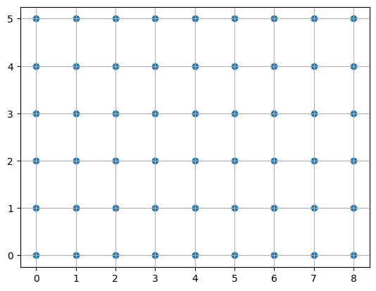
x, y = np.meshgrid(range(9), range(6)) #world point격자 생성(체스보드는 2D로 보기때문에 2D 월드좌표계)
world_points = np.hstack((x.reshape(54, 1), y.reshape(54, 1))).astype(np.float32) #(x,y)좌표 쌍 생성
world_points = world_points*21.5 # rectangular size 21.5를 곱해 실제 체스보드처럼
world_points = np.asarray(world_points)
images_points = []
homography_matrices = []
for imagepath in image_path:
image = cv2.imread(imagepath)
#scale_percent = 0.3 # 변환시킬 수도 있음
#height = int(image.shape[0] * scale_percent)
#width = int(image.shape[1] * scale_percent)
#dim = (width, height)
gray = cv2.cvtColor(image, cv2.COLOR_BGR2GRAY) #변환하지 않아도 되지만 약간의 연산량 차이가 날수도?
ret, corners = cv2.findChessboardCorners(gray, (9, 6), None) # ret: 찾을 수 있다면 True or False,
# opencv 함수활용해 코너 찾는다
if ret == True:
corners = corners.reshape(-1, 2)
#gray = cv2.drawChessboardCorners(gray, (9, 6), corners, ret)
homography_matrix = computeHomography(corners, world_points) #corner, world point활용해 homography 행렬
images_points.append(corners)
homography_matrices.append(homography_matrix)
updateVMatrix(homography_matrix, V)
#cv2_imshow(gray)
#cv2.waitKey(500)
#cv2.destroyAllWindows()
V = np.asarray(V)
b = getBMatrix(V)
K, lamda = getCalibMatrix(b)
error = 0
for image_points, homograph_matrix in zip(images_points, homography_matrices):
R, t = getExtrinsicParams(K, lamda, homography_matrix) #extrinsic parameter 구하기
reprojection_error = getReprojectionError(image_points, world_points, K, R, t)
error += reprojection_error #에러계산
error /= (13*9*6)
print('ERROR : {}'.format(error))
init = [K[0, 0], K[1, 1], K[0, 2], K[1, 2], K[0, 1], 0, 0] #(0, 0)은 왜곡계수, 그러나여기서는 0가정
res = opt.least_squares(fun = optimizationCostFunction, x0 = init, method = 'lm',
args = [lamda, images_points, world_points, homography_matrices])
K_opt = np.zeros(shape = (3, 3))
K_opt[0, 0], K_opt[1, 1], K_opt[0, 2], K_opt[1, 2], K_opt[0, 1], K_opt[2, 2] = res.x[0], res.x[1], res.x[2], res.x[3], res.x[4], 1
#최적화
k1_opt, k2_opt = res.x[5], res.x[6]
print('CALIBRATION MATRIX AFTER OPTIMIZATION : {}'.format(K_opt))
print('DISTIORTION COEFFICIENT AFTER OPTIMIZATION : {}'.format(k1_opt, k2_opt))
error_opt = 0
optimized_points = []
for image_points, homography_matrix in zip(images_points, homography_matrices):
R, t = getExtrinsicParams(K_opt, lamda, homography_matrix)
reprojection_error, reprojected_points = getReprojectionErrorOptimized(image_points, world_points, K_opt, R, t, k1_opt, k2_opt)
optimized_points.append(reprojected_points)
error_opt = error_opt + reprojection_error
error_opt = error_opt/(13*9*6)
print("\nMean Reprojection error after optimization: \n{}".format(error_opt[0]))
displayReprojectedPoints(images_points, optimized_points, image_path)
x, y = np.meshgrid(range(9), range(6)) #world point격자 생성(체스보드는 2D로 보기때문에 2D 월드좌표계)
world_points = np.hstack((x.reshape(54, 1), y.reshape(54, 1))).astype(np.float32)  #(x,y)좌표 쌍 생성
world_points = world_points*21.5 # rectangular size 21.5를 곱해 실제 체스보드처럼
world_points = np.asarray(world_points)
world 좌표계 생성. 사각형의 길이가 21.5mm라 기존 격자점에 곱해준다.
images_points = []
homography_matrices = []

for imagepath in image_path:
  image = cv2.imread(imagepath)
  #scale_percent = 0.3  # 변환시킬 수도 있음
  #height = int(image.shape[0] * scale_percent)
  #width = int(image.shape[1] * scale_percent)
  #dim = (width, height)

  gray = cv2.cvtColor(image, cv2.COLOR_BGR2GRAY) #변환하지 않아도 되지만 약간의 연산량 차이가 날수도?

  ret, corners = cv2.findChessboardCorners(gray, (9, 6), None) # ret: 찾을 수 있다면 True or False,
        # opencv 함수활용해 코너 찾는다
  if ret == True:
    corners = corners.reshape(-1, 2)
    #gray = cv2.drawChessboardCorners(gray, (9, 6), corners, ret)
corners 의 크기: (54, 1, 2) --> (54, 2)
ret : corners 다 찾으면 True, 그렇지 않으면 False
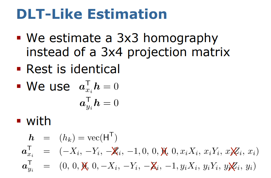
homography_matrix = computeHomography(corners, world_points) #corner, world point활용해 homography 행렬def computeHomography(corners, world_points):
src = np.asarray(world_points)
dst = np.asarray(corners)
homography, _ = cv2.findHomography(src, dst) #_ 값은 mask값. 여기서는 별로 필요없는듯?
#n = 20
#src = np.asarray(world_points[: n]) # world
#dst = np.asarray(corners[: n]) # image
#P = np.zeros((2*n, 9)) # homography는 3x3행렬이므로
#i = 0
#for (srcpt, dstpt) in zip(src, dst):
#x, y, x_dash, y_dash = srcpt[0], srcpt[1], dstpt[0], dstpt[1]
#P[i][0], P[i][1], P[i][2] = -x, -y, -1 #자료 21p
#P[i+1][0], P[i+1][1], P[i+1][2] = 0, 0, 0
#P[i][3], P[i][4], P[i][5] = 0, 0, 0
#P[i+1][3], P[i+1][4], P[i+1][5] = -x, -y, -1
#P[i][6], P[i][7], P[i][8] = x*x_dash, y*x_dash, x_dash
#P[i+1][6], P[i+1][7], P[i+1][8] = x*y_dash, y*y_dash, y_dash
#i = i+2
#_, _, vh = np.linalg.svd(P, full_matrices=True) #Direct Linear transform #환기님 자료 23p
#h = vh[-1:] #마지막 행만 추출 이유는..?
#h.resize((3, 3))
#homography = h/h[2, 2]
return homography처음 homography 행렬은 intrinsic, extrinsic 행렬이 아닌 2개의 이미지 코너 좌표들만을 활용하여 구한다.
    images_points.append(corners)
    homography_matrices.append(homography_matrix)

    updateVMatrix(homography_matrix, V)
def updateVMatrix(H, V): #자료 42p
    v_12 = [H[0][0]*H[0][1], (H[0][0]*H[1][1] + H[1][0]*H[0][1]), H[1][0]*H[1][1],
            (H[2][0]*H[0][1] + H[0][0]*H[2][1]), (H[2][0]*H[1][1] + H[1][0]*H[2][1]), H[2][0]*H[2][1]]

    # print v_12
    # v11 - v22 한번에 계산
    trm1 = H[0][0]*H[0][0] - H[0][1]*H[0][1]
    trm2 = 2*(H[0][0]*H[1][0] - H[0][1]*H[1][1])
    trm3 = H[1][0]*H[1][0] - H[1][1]*H[1][1]
    trm4 = 2*(H[2][0]*H[0][0] - H[0][1]*H[2][1])
    trm5 = 2*(H[2][0]*H[1][0] - H[1][1]*H[2][1])
    trm6 = H[2][0]*H[2][0] - H[2][1]*H[2][1]

    v_1122 = []
    v_1122.append(trm1)
    v_1122.append(trm2)
    v_1122.append(trm3)
    v_1122.append(trm4)
    v_1122.append(trm5)
    v_1122.append(trm6)

    # print v_1122

    V.append(v_12)
    V.append(v_1122)

    # print V
    # print "\n \n"
V매트릭스에 대해서 다른 설명을 찾을 수 없었는데 개인적인 이해로는 '두 이미지의 코너값을 이용해서 구한 homography 행렬을 이용하여 V라는 행렬을 찾을 수 있다' 로 이해.
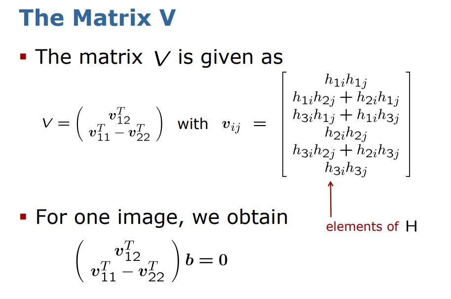
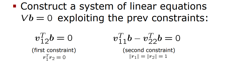
b = getBMatrix(V)추가적으로 V라는 매트릭스를 통해서 b라는 matrix를 구하는데, 구하는 이유는 기존의 식에서 Vb = 0 라는 제약식을 얻을 수 있기 때문이다.
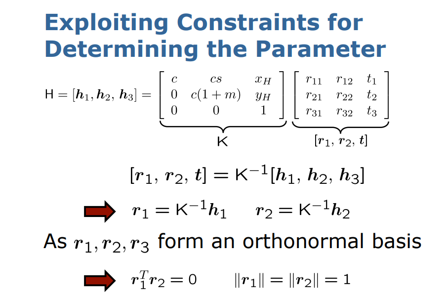
기존의 식인데 조금 변형을 가해주면 r1, r2의 크기가 1인 것을 활용하여, r1^T * r2 = 0 이라는 값을 얻는다.
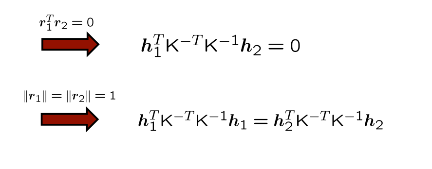
위에서 얻은 제약식을 전개한 모습이다.
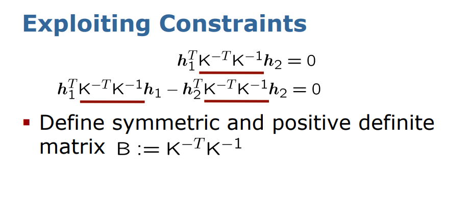
이러한 두개의 제약식을 통해 K^-T * K^-1 의 행렬 곱을 B라는 행렬로 치환한 모습이다.
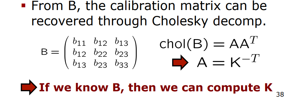
그리고 B라는 행렬은 정방행렬, 대칭행렬이기 때문에 Cholesky 분해를 통해 B = A*A^-T라는 값을 얻는데 A(A는 하삼각행렬)값을 구하면 K(intrinsic parameter)값을 구할 수 있다. 이 과정에서 b라는 값은 위에서 구한 V행렬을 통해 구할 수 있다.
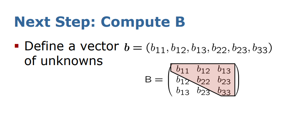
결국 두 이미지의 코너 좌표들을 통해 초기 homography 행렬을 구한 후, V라는 행렬을 구한 후, V*b = 0 이라는 제약식을 통해서 B라는 행렬을 얻으면 K값을 얻을 수 있다.
def getBMatrix(V):
    _, _, vh = np.linalg.svd(V, full_matrices=True)
    #  Vb = 0 #자료 43페이지 ~ 45페이지
    b = vh[-1:]
    return b
b행렬은 V행렬에 특이값분해를 통해 얻을 수 있다. 왜 마지막 행만 사용하는지..?
K, lamda = getCalibMatrix(b)def getCalibMatrix(b): #calibration matrix구하는 함수
#b : 투영행렬(projection matrix)
v = (b[0][1]*b[0][3] - b[0][0]*b[0][4])/(b[0][0]*b[0][2] - b[0][1]**2)
lamda = b[0][5] - (b[0][3]**2 +
v*(b[0][1]*b[0][3] - b[0][0]*b[0][4]))/b[0][0]
fx = math.sqrt(lamda/b[0][0])
fy = math.sqrt(lamda*b[0][0]/(b[0][0]*b[0][2] - b[0][1]**2))
skew = (-1*b[0][1]*fx**2*fy)/(lamda)
u = (skew*v)/fy - (b[0][3]*fx**2)/lamda
print("u = {}\nv = {}\nlamda = {}\nfx = {}\nfy = {}\nskew = {}\n".format(
u, v, lamda, fx, fy, skew))
K = np.array([[fx, skew, u], [0, fy, v], [0, 0, 1]])
return K, lamda위에서 설명한 것처럼 b행렬을 통해 K행렬을 구하는 함수이다. b행렬의 각 원소가 어떤 기하학적인 의미를 가지는지 모르겠는데 이렇게 구현을 한다..
error = 0

for image_points, homograph_matrix in zip(images_points, homography_matrices):
  R, t = getExtrinsicParams(K, lamda, homography_matrix) #extrinsic parameter 구하기

  reprojection_error = getReprojectionError(image_points, world_points, K, R, t)

  error +=  reprojection_error #에러계산
기존에 구했던 homography 행렬과 K를 이용해 extrinsic parameter구할 수 있다.
def getExtrinsicParams(K, lamda, homography_matrix):
K_inv = np.linalg.inv(K) #K의 역행렬을 구한다(여기서 K는 intrinsic parameters matrix)
r1 = np.dot(K_inv, homography_matrix[:, 0]) #K 역행렬과 변환행렬의 첫번째 열 곱셈.
lamda = np.linalg.norm(r1, ord=2),
r1 = r1/lamda #정규화
r2 = np.dot(K_inv, homography_matrix[:, 1]) #K 역행렬과 변환행렬의 두번째 열 곱셈
r2 = r2/lamda #정규화
t = np.dot(K_inv, homography_matrix[:, 2])/lamda #K 역행렬과 변환행렬의 세번째 열 곱셈
r3 = np.cross(r1, r2) #외적을 통해 z축
R = np.asarray([r1, r2, r3]) #회전행렬
R = R.T
# t = np.array([t])
# t = t.T
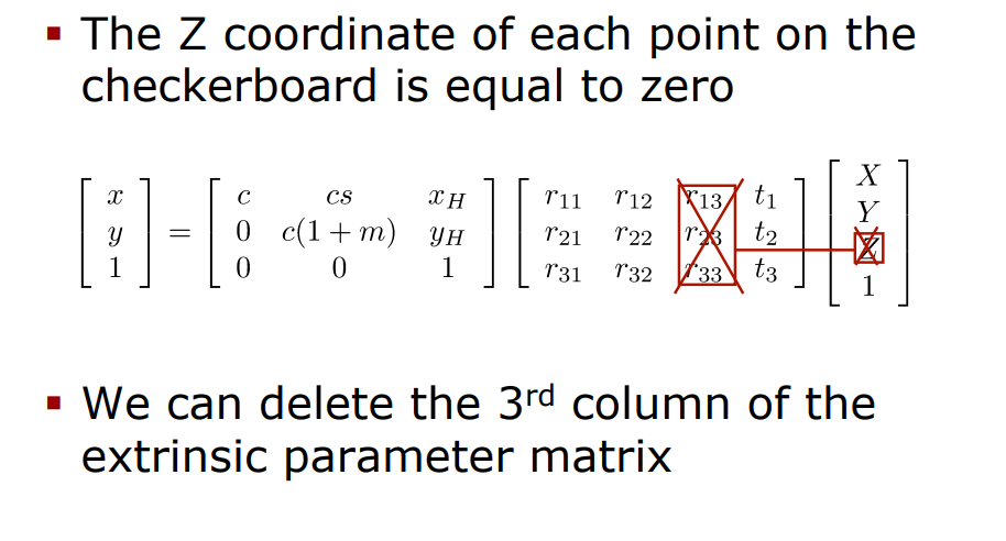
return R, t #회전행렬과 평행이동행렬기존 K *[R|t] = H, [R|t] = K^-1 * H이므로 각 K의 역행렬을 구해 R 의 열백터를 구해준다. 여기서 체스보드 판은 2D이므로 r3는 0일 것이다(개인적인생각).
이제 파라미터들을 다 구했으니 reprojection error를 구할 차례이다.
def getReprojectionError(image_points, world_points, A, R, t): #오차계산
    error = 0
    augment = np.zeros((3, 4))
    augment[:, :-1] = R
    augment[:, -1] = t

    N = np.dot(A, augment)

    for pt, wrldpt in zip(image_points, world_points):
        M = np.array([[wrldpt[0]], [wrldpt[1]], [0], [1]]) #world point
        realpt = np.array([[pt[0]], [pt[1]], [1]]) #image point
        projpt = np.dot(N, M) # 투영된 이미지
        projpt = projpt/projpt[2]
        diff = realpt - projpt
        error = error + np.linalg.norm(diff, ord=2) #에러계산. l2 norm사용

    return error
world point를 image plane에 투영을 하고 이에 대한 오차를 계산한다.
init = [K[0, 0], K[1, 1], K[0, 2], K[1, 2], K[0, 1], 0, 0] #(0, 0)은 왜곡계수, 그러나여기서는 0가정
res = opt.least_squares(fun = optimizationCostFunction, x0 = init, method = 'lm',
                        args = [lamda, images_points, world_points, homography_matrices])

K_opt = np.zeros(shape = (3, 3))
K_opt[0, 0], K_opt[1, 1], K_opt[0, 2], K_opt[1, 2], K_opt[0, 1], K_opt[2, 2] = res.x[0], res.x[1], res.x[2], res.x[3], res.x[4], 1
#최적화
k1_opt, k2_opt = res.x[5], res.x[6]
여기서 초기값을 할당해주고, method는 loss를 최소화하는 알고리즘인데 3가지가 있다.
trf (기본값): Trust Region Reflective algorithm, particularly suitable for large sparse problems with bounds. Generally robust method.
dogbox : dogleg algorithm with rectangular trust regions, typical use case is small problems with bounds. Not recommended for problems with rank-deficient Jacobian.
lm : Levenberg-Marquardt algorithm as implemented in MINPACK. Doesn’t handle bounds and sparse Jacobians. Usually the most efficient method for small unconstrained problems.
우리가 최적화해야 하는 함수는 다음과 같다.
def optimizationCostFunction(init, lamda, images_points, world_points, homography_matrices): #최소화 해야하는 값
    K = np.zeros(shape=(3, 3)) #초기 매개변수 활용해 init 값 넣기위한 행렬
    K[0, 0], K[1, 1], K[0, 2], K[1, 2], K[0, 1], K[2, 2] = init[0], init[1], init[2], init[3], init[4], 1
    k1, k2 = init[5], init[6] #왜곡계수
    u0, v0 = init[2], init[3] #좌표

    reprojection_error = np.empty(shape=(1404), dtype=np.float64) #투영값 저장위한 array. 702쌍 최적화
    i = 0 #모든 지점에서 변환이 생기기 때문에 homography matrix는 다수 존재
    for image_points, homography_matrix in zip(images_points, homography_matrices):
        R, t = getExtrinsicParams(K, lamda, homography_matrix) #intrinsic parameter와 homography 활용해 R, t(R: 3x3 행렬)

        augment = np.zeros((3, 4))
        augment[:, :-1] = R
        augment[:, -1] = t #augment 행렬에 R, t를 넣어준다.

        for pt, wrldpt in zip(image_points, world_points): # 각 쌍들에 대한 오차 계산
            M = np.array([[wrldpt[0]], [wrldpt[1]], [0], [1]]) #world 좌표게
            ar = np.dot(augment, M) #결과값: 3x1
            ar = ar/ar[2] # w값으로 나누어준다
            x, y = ar[0], ar[1] #픽셀 좌표계

            U = np.dot(K, ar)
            U = U/U[2]
            u, v = U[0], U[1] #정규좌표계

            t = x**2 + y**2        #  Q. 왜 이값을 이용하는지는 ?
            u_dash = u + (u-u0)*(k1*t + k2*(t**2)) #수정된 값
            v_dash = v + (v-v0)*(k1*t + k2*(t**2))

            reprojection_error[i] = pt[0]-u_dash #각각의 에러값을 넣는다
            i += 1
            reprojection_error[i] = pt[1]-v_dash
            i += 1

    return reprojection_error
그리고 최적화를 끝낸 이후 또 다시 error를 체크해본다.
error_opt = 0
optimized_points = []
for image_points, homography_matrix in zip(images_points, homography_matrices):
  R, t = getExtrinsicParams(K_opt, lamda, homography_matrix)

  reprojection_error, reprojected_points = getReprojectionErrorOptimized(image_points, world_points, K_opt, R, t, k1_opt, k2_opt)
  optimized_points.append(reprojected_points)

  error_opt = error_opt + reprojection_error

error_opt = error_opt/(13*9*6)
print("\nMean Reprojection error after optimization: \n{}".format(error_opt[0]))

displayReprojectedPoints(images_points, optimized_points, image_path)
CALIBRATION MATRIX AFTER OPTIMIZATION : [[1.31820173e+03 2.52428320e+03 8.02006603e+02]
 [0.00000000e+00 6.95974739e+02 1.35090505e+03]
 [0.00000000e+00 0.00000000e+00 1.00000000e+00]]
DISTIORTION COEFFICIENT AFTER OPTIMIZATION : 0.0005494239814192967

Mean Reprojection error after optimization:
0.7365561871552351
https://github.com/JiWoongCho1/Project/blob/main/Calibration/Calibration.ipynb
GitHub - JiWoongCho1/Project: 머신러닝 및 알고리즘 프로젝트
머신러닝 및 알고리즘 프로젝트. Contribute to JiWoongCho1/Project development by creating an account on GitHub.
github.com
'Graphics' 카테고리의 다른 글
| Epipolar Geometry 공부해보기 (0) | 2023.04.18 |
|---|---|
| Camera calibration을 위한 여러가지 용어 정리 (0) | 2023.04.13 |

